5.1 Nurbs Curves

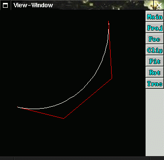
In Example 4 a cubic nurbs curve with a clamped, normalized knot vector is created. The control points of the curve are also shown as a polyline.

Figure 5.1 shows the curve in white and the polyline in red.

Example 4: (taken from: data/examples/nurbcurv1.dat (7.21))

cpts = ((0,0,0,1), (0.25, 0.3, 0, 1),  (0.75, 0.3, 0, 1),  (1,0,0,1));
curv1 = NURBCURV( 
  ( 0, 0, 0, 0, 1, 1, 1, 1 ),
  cpts
);
poly1 = POLYLINE_H3(cpts);

SCENEROOT = SCENENODE( (), (ATTRIBS(LINECOLOR((1,0,0,1)))), (curv1,poly1) );

Figure 5.1: Cubic Nurbs Curve with clamped knot vector

In the Example 5 the clamped knotvector is replaced by an open one. The resulting curve is shown in Figure 5.2.

Example 5: (taken from: data/examples/nurbcurv2.dat (7.22))

cpts = ((0,0,0,1), (0.25, 0.3, 0, 1),  (0.75, 0.3, 0, 1),  (1,0,0,1));
curv1 = NURBCURV( 
  ( 1, 2, 3, 4, 5, 6, 7, 8 ),
  cpts
);

Figure 5.2: Cubic Nurbs Curve with open knot vector

In Example 6 a quadratic curve is created, which has the same control point vector as the cubic curve in figure 5.1. It is shown in Figure 5.3.

Example 6: (taken from: data/examples/nurbcurv3.dat (7.23))

cpts = ((0,0,0,1), (0.25, 0.3, 0, 1),  (0.75, 0.3, 0, 1),  (1,0,0,1));
curv1 = NURBCURV( 
  ( 0., 0., 0., 0.5, 1., 1., 1. ),
  cpts
);

Figure 5.3: Quadratic Nurbs Curve