5.7 Global and Local Interpolation with Nurbs Curves

In this section two examples of global and local curve interpolation (see Piegl/ Tiller 4.3) are given. Both examples use the same data point set.

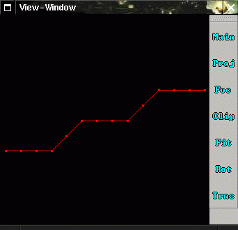
The data point set is shown in Figure 5.13 (the code with which Figure 5.13 was created can be found in Example 14).

Example 14: (taken from: data/examples/curv_testcase.dat (7.5))

dpts1 =
  ((0,0,0),(1,0,0),(2,0,0),(3,0,0), (4,0,1), 
   (5,0,2),(6,0,2),(7,0,2),(8,0,2), (9,0,3),
   (10,0,4),(11,0,4),(12,0,4),(13,0,4));

lin1 = POLYLINE( dpts1 );
pts1 = POINTS( dpts1 );

SCENEROOT = SCENENODE ( (), (), (lin1,pts1) );

Figure 5.13: Testcase for Curve Interpolation/Approximation

In Example 15 the point set is interpolated with a curve of degree 3, using Global Interpolation. The result is shown in Figure 5.14.

In Example 16 the point set is interpolated with a cubic curve, using Local Cubic Interpolation. The result is shown in Figure 5.15. The resulting curve is not so smooth as that from Example 15 (it is only $C^1$ continuous), but it is closer to the polyline through the data points. It is also possible, to make the Local Cubic Interpolation algorithm corner preserving (when doing so in the example below, the created curve exactly looks like the polyline through the data points depicted in Figure 5.13).

Figure 5.14: Global Interpolation Curve

Figure 5.15: Local Cubic Interpolation Curve

Example 15: (taken from: data/examples/nubgic1.dat (7.15))

curv1 = NUBGIC( 
  3,       /* degree */
           /* vector of data points: */
  dpts1
);
pts1 = POINTS( dpts1 );
lin1 = POLYLINE( dpts1 );
SCENEROOT = SCENENODE ( (), (), (pts1,curv1,lin1) );

Example 16: (taken from: data/examples/nublbic1.dat (7.17))

curv1 = NUBLBIC( 
  0,       /* preserve corner flag */
           /* vector of data points: */
  dpts1
);