5.8 Global Approximation with Nurbs Curves

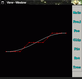
In Example 17 the point set from the previous section is approximated by a curve with degree 3 and 4 control points, using Global Approximation (see Piegl/ Tiller 4.3). The result is shown in Figure 5.16.

Example 17: (taken from: data/examples/nubgac1.dat (7.11))

curv1 = NUBGAC( 
  3,       /* degree */
  4,       /* number of control points */
           /* vector of data points: */
  dpts1 = 
  ((0,0,0),(1,0,0),(2,0,0),(3,0,0), (4,0,1), 
   (5,0,2),(6,0,2),(7,0,2),(8,0,2), (9,0,3),
   (10,0,4),(11,0,4),(12,0,4),(13,0,4))
);

pts1 = POINTS( dpts1 );
lin1 = POLYLINE( dpts1 );
SCENEROOT = SCENENODE ( (), (), (pts1,curv1,lin1) );

Figure 5.16: Global Approximation Curve, using degree 3 and 4 control points

In Example 17 and 18 8 and 11 control points are used. The results are shown in Figures 5.17 and 5.18.

One has to keep in mind that in this algoritm only the error at the data points is minimized (in the least squares sense). So it is well possible that the curve does strange things between data points in order to reduce that error, especially when using a pathological data set like the above with colinear points (see Figure 5.18).

Figure 5.17: Global Approximation Curve, using degree 3 and 8 control points

Figure 5.18: Global Approximation Curve, using degree 3 and 11 control points

Example 18: (taken from: data/examples/nubgac2.dat (7.12))

curv1 = NUBGAC( 
  3,       /* degree */
  8,       /* number of control points */
           /* vector of data points: */
  dpts1
);

Example 19: (taken from: data/examples/nubgac3.dat (7.13))

curv1 = NUBGAC( 
  3,       /* degree */
  11,       /* number of control points */
           /* vector of data points: */
  dpts1
);