5.11 Iso Surfaces and Marching Cube

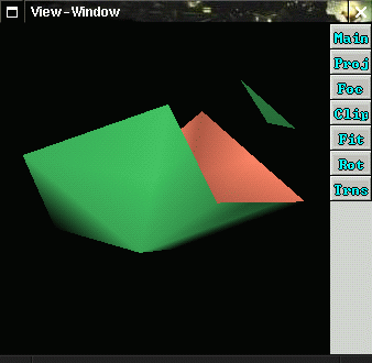
The regions of a 3D grid of values where a sign change occurs can be shown with the marching cube algorithm.

In Example 27 a grid is created which ranges from -2 to 2 in the x, y and z direction with a stepwidth of 1 (=> 5*5*5 values), and is displayed with the marching cube algorithm. The result is shown in Figure 5.29.

Example 27: (taken from: data/examples/grid3_1.dat (7.6))

grid1 = GRID3( 
  (-2.,1.), 
  (-2.,1.), 
  (-2.,1.),
  (
  ((1.0, 1.0, 1.0, 1.0, 1.0),
  (1.0, 1.0, 1.0, 1.0, 1.0),
  (1.0, 1.0, 1.0, 1.0, 1.0),
  (1.0, 1.0, 1.0, 1.0, 1.0),
  (1.0, 1.0, 1.0, 1.0, 1.0)),

  ((1.0, 1.0, 1.0, 1.0, 1.0),
  (1.0, 1.0, 1.0, 1.0, 1.0),
  (1.0, -1.0, -1.0, 1.0, 1.0),
  (1.0, -1.0, -1.0, 1.0, 1.0),
  (1.0, 1.0, 1.0, 1.0, 1.0)),

  ((1.0, 1.0, 1.0, 1.0, 1.0),
  (1.0, 1.0, 1.0, 1.0, 1.0),
  (1.0, 1.0, -1.0, 1.0, 1.0),
  (1.0, -1.0, 1.0, 1.0, 1.0),
  (1.0, 1.0, 1.0, 1.0, 1.0)),

  ((1.0, 1.0, 1.0, 1.0, 1.0),
  (1.0, 1.0, 1.0, 1.0, 1.0),
  (1.0, -1.0, 1.0, 1.0, 1.0),
  (1.0, 1.0, -1.0, 1.0, 1.0),
  (1.0, 1.0, 1.0, 1.0, 1.0)),

  ((1.0, 1.0, 1.0, 1.0, 1.0),
  (1.0, 1.0, 1.0, 1.0, 1.0),
  (1.0, 1.0, 1.0, 1.0, 1.0),
  (1.0, 1.0, 1.0, 1.0, 1.0),
  (1.0, 1.0, 1.0, 1.0, 1.0))
  )
);
march1 = MARCHCUBE( grid1 );
SCENEROOT = SCENENODE ( 
  (), 
  (ATTRIBS(front1,back1)), 
  (march1)
);

Figure 5.29: Areas of a 3D grid where a sign change occurs

In Example 28, Example 29, Example 30 and Example 31 first functions are defined, which have the 3 dimensional space as their domain, then values of these functions are sampled at a regular grid of (x, y, z) locations, and finally this grid is displayed via the marching cube algorithm.

Please see Section 6.6 and Section 6.7 for the definition of the keywords GRID3 (6.6.3), GRIDEVAL3 (6.6.4), FORMULA3 (6.6.2) and MARCHCUBE (6.7.1).

Example 28 visualizes the iso surface $F(x,y,z) = 0$ of the function $F(x,y,z) = x^2 + y^2 + z^2 - 1$. A very coarse sample grid of only 11*11*11 points was used. The result is shown in Figure 5.30.

Example 28: (taken from: data/examples/formula3_1.dat (7.7))

form1 = FORMULA3( "x*x + y*y + z*z - 1;", () );
grid1 = GRIDEVAL3( (-2.,10,0.4), (-2.,10,0.4), (-2.,10,0.4), form1 );
march1 = MARCHCUBE( grid1 );

Figure 5.30: Sphere as a Iso Surface

Example 29 visualizes the iso surface $F(x,y,z) = 0$ of the function $F(x,y,z) = sin(x)$. The result is shown in Figure 5.31. As expected inside and outside changes at $x = 0, pi, 2*pi$.

Example 29: (taken from: data/examples/formula3_2.dat (7.8))

form1 = FORMULA3( "sin(x);", () );
grid1 = GRIDEVAL3( ( -0.5,50,0.14), (-2.5,5,1.0), (-2.5,5,1.0), form1 );
march1 = MARCHCUBE( grid1 );

Figure 5.31: Iso Surface $sin(x) = 0$

Example 30 visualizes the iso surface $F(x,y,z) = 0$ of the quadratic polynom

$F(x,y,z)$	$=$	$0.0260516*x^2 + 0.028689*y^2 + 0.0100072*z^2$
		$- 0.057882*x*y + 0.0217817*x*z - 0.0187733*y*z$
		$- 0.0812969*x + 0.086143*y + 0.00396285*z - 1.0$

The coefficients for this polynom were calculated by minimizing

$1$	$=$	$a_1*x^2 + a_2*y^2 + a_3*z^2$
		$+ a_4*x*y + a_5*x*z + a_6*y*z$
		$+ a_7*x + a_8*y + a_9*z$

for a set of data points with least squares. The result is shown in Figure 5.32.

Example 30: (taken from: data/examples/formula3_3.dat (7.9))

form1 = FORMULA3( "0.0260516*x*x + 0.028689*y*y + 0.0100072*z*z
                  - 0.057882*x*y + 0.0217817*x*z - 0.0187733*y*z
                  - 0.0812969*x + 0.086143*y + 0.00396285*z - 1.0;", () );
grid1 = GRIDEVAL3( (-30.,50,1.2), (-30.,50,1.2), (-30.,50,1.2), form1 );
march1 = MARCHCUBE( grid1 );

Figure 5.32: Quadratic Polynom approximating a set of data points

In Example 31 the term $0.0260516*x^2$ in Example 1003 was replaced with the term $0.0260516*x^2*z^2$, the result is shown in Figure 5.33.

Example 31: (taken from: data/examples/formula3_4.dat (7.10))

form1 = FORMULA3( "0.0260516*x*x*z*z + 0.028689*y*y + 0.0100072*z*z
                   - 0.057882*x*y + 0.0217817*x*z - 0.0187733*y*z
                   - 0.0812969*x + 0.086143*y + 0.00396285*z - 1.0;", () );
grid1 = GRIDEVAL3( (-30.,50,1.2), (-30.,50,1.2), (-30.,50,1.2), form1 );
march1 = MARCHCUBE( grid1 );

Figure 5.33: A Nice Implicitly Defined Surface